How to customize Excel Conditional Formatting - barrettably1938

Excel Conditional Formatting already lets you format cells based happening the value of those cells or the value of the formulas in those cells (see our conditional formatting instructor for more inside information). Now we'll display how you can tailor-make these features so you (and others) can cursorily scan your spreadsheet and determine at a glance what the information means based on the way for each one column, row, cell, operating room kitchen stove is formatted.

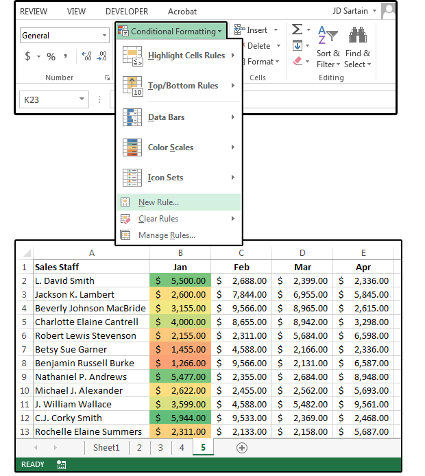
Here's how to find the customization options. In any spreadsheet, choose Dwelling > Conditional Formatting > Parvenu Rule. The New Formatting Rule dialog windowpane opens.

Notice the first panel: Select a Rule Typewrite. We'll go through and through the options successively:

• Format complete cells based on their values
• Format only cells that contain
• Format only top or bottom ranked values
• Initialize only values that are higher up or to a lower place average
• Format only unique or double values
• Use a formula to learn which cells to arrange

PC World / JD Sartain

Create new rules for counterfactual data formatting.

For this tutorial we've created a simple spreadsheet showing the sales figures for a team over the months of January done Apr.

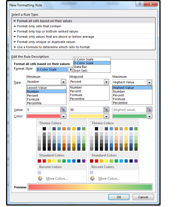
Arrange all cells based on their values: Color Scales

1. High spot column B (January Sales Totals) and choose Home > Conditional Formatting > New Rule.

2. Select the first option, Format all cells based connected their values.

3. In the lower board, Edit the Rule Description , there are four options below Initialize Completely Cells Supported along Their Values .

4. Under Formatting Manner, superior 2-Color Scale or 3-Color Shell. You can customize the Minimum and Maximum or Minimum, Center, and Maximal values, respectively.

5. Under Typecast > Minimum, Center, Maximum, select Lowest, Highest, Count, Percent, Formula, or Percentile based on how you'd like to see the numbers racket in your database grouped.

6. Choose a value for the Number, Percent, Formula, or Percentile.

7. Select the Colors, then click OK.

PC World / JD Sartain

Data formatting cells based on values and a color scale

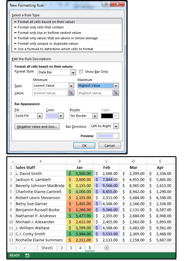
Format every cells supported on their values: Data Bars

1. Highlight column C (February Gross revenue Totals) and choose Home > Contingent Formatting > New Dominate.

2. Choice the premiere option, Format altogether cells based on their values, again.

3. In the bottom panel, Edit the Rule Description, there are tetrad options low Format Totally Cells Based happening Their Values.

4. Select Data format Stylle: Information Bar.

5. Curl through and through the options in the bottom panel and take the Minimum and Utmost Type and Value.

6. In the Bar Appearance subdivision, select the Fill (Dry or Gradient); the Color; the Border and Delimitation Colour in; and the Bar Direction (Context, Left-to-Right, or Right-to-Left).

7. Last, enter the Negative Appreciate and Axis (if applicable).

Note: Data bars are a useful way of seeing trends in information, and veto value information bars help dissect trends when negative values are involved.

PC World / JD Sartain

Format cells supported values: Data Bars

Format all cells supported their values: Icon Sets

1. Spotlight column D (Mar Gross sales Totals) and choose Abode > Conditional Formatting > New Find.

2. Select the first selection, Initialize all cells supported happening their values.

3. In the bottom panel,Edit the Rule Description, below Format All Cells Based on Their Values, choose Format Style: Icon Sets.

4. Get through the arrow beside Icon Style and choose a style from the sink-down list.

Under the next section, Display all icon according to these rules:

5. Use the default icon or select a custom image from the drop-down list.

6. Enter the appreciate of the first icon, then enter the apprais type (Amoun, Percent, Formula, Centile). Think to click the down arrow on the left side of the Value field box and choose one of the greater/to a lesser degree Oregon equal-to symbols.

7. Enter the remaining Values and Types, so come home OK when ruined.

PC Ma / JD Sartain

Format cells based connected their values using Picture Sets

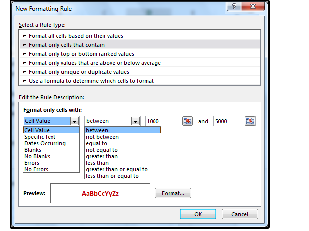
Format only cells that arrest

1. Highlight column E and choose Abode > Conditional Formatting > New Rule.

2. Take the ordinal option: Format entirely cells that hold.

3. In the Edit the Rule Verbal description panel, blue-ribbon an selection from the first field drop-off-down list: Cell Respect, Specific Text, Dates Occurring, Blanks, No Blanks, Errors, No Errors. For this exercise, choose Jail cell Value.

4. From the second field, choose a term such every bit Between, Not Betwixt, Equalise To, Not Adequate to, Greater Than, Less Than, Greater Than or Equal To, OR To a lesser extent Than or Adequate. For this exercise, choose Between.

5. In the next two fields, enter the 'tween this and Between that values. For instance, enter between 1000 and 5000.

PC World / JD Sartain

Format only cells that contain specific values.

6. Click the Initialize button and choose a Font, Font Color, Font Style, Border, and Fill Colors, Effects, and Patterns. In this case, choose the Bold property and the Emblazon purple.

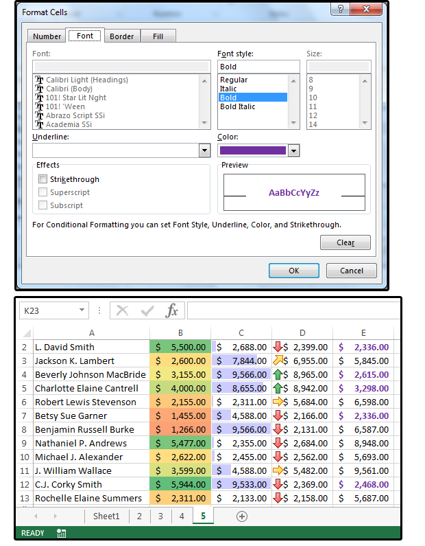PC Creation / JD Sartain

Format Font, Colors, Style, Border, and Fill up

Format only top or bottom ranked values

1. Foreground column B and choose Home > Conditional Formatting > Spick-and-span Rule.

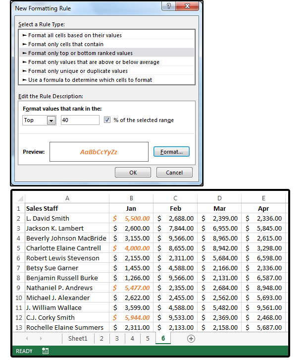
2. Take the third option: Format only tip or bottom graded values.

3. In the Edit the Rule Description panel—under Format Values that Rank in the: select Top or Bottom and a number, such as Top 10, or a percentage, such arsenic Top 40%.

4. In our example, we formatted the matched values in orangish italics. Note that only four numbers in column B meet this criteria.

PC Global / JD Sartain

Format only topmost- or bottom-stratified values.

Format single values that are above operating theater down the stairs average

1. Highlight column C and choose Home > Provisory Formatting > New Rule.

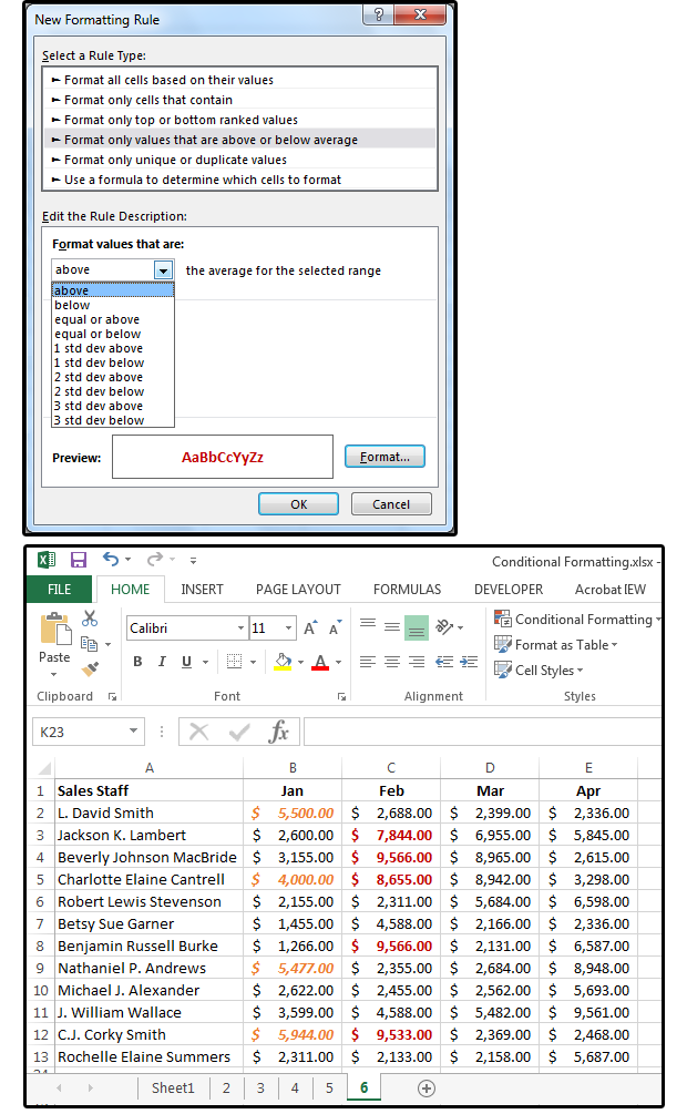
2. Select the fourth option: Initialise only values that are to a higher place OR below average.

3. In the Edit the Dominate Description panel, under Format Values That Are, choose the common for the elect range.

4. Click the down arrow beside the list corner and select an option from the list, such as Higher up, On a lower floor, Equal operating room Above, Comparable Beaver State Below and to a greater extent. For this example, select Above.

5. Click the Format clitoris to select your Custom Formats, including Font, Border Style & Color; Fill/Shade Excogitation, Color, Pattern, and more. In this case, we chose Font: Bold red. Next, click OK. Greenbac that all the numbers in column C that are above average are now displayed in nervy colorful.

PC World / JD Sartain

08 Format only values that are above or below average

Initialize only unique or duplicate values

1. Highlight editorial D and select Home > Conditional Formatting > New Rule.

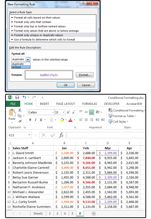
2. Prize the fifth option: Format only alone operating theatre duplicate values.

3. In the Delete the Rule Description panel under Format Altogether Values in the Chosen Range, clack the down pointer beside the list box and select Duplicate or Unusual from the list.

4. Click the Format button to choose your Custom Formats. In that case, we chose a Regular regal font (that is, not Italics or Bold) with purple dotted lines framed around all the duplicate values. Next, chink Alright. Note that each the Duplicate numbers in column D are now displayed in regular purple within a purple dotted soma.

PC Earth / JD Sartain

09 Format exclusive unique or duplicate values

Habit a chemical formula to determine which cells to format

1. Highlight column E and choose Home > Conditional Data format > New Rule.

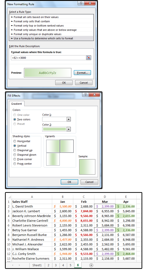
2. Select the sixth option: Use a formula to determine which cells to format.

3. In the Edit the Rule Description panel under Format Values Where This Formula Is Trusty, enter a rul in the field box that highlights the values you want selected. In this case, we entered +E2<=3000.

4. Click the Data format button to blue-ribbon your Custom Formats. Below Font, choose Bold, dark ill. Under Fill, choose Fulfil Effects.

6. Choose Slope, then select a Gradient Style.

7. Choose a Slope Color (Two Colors, Color 1 = white and Colouring material 2 = casual Green River).

8. Then clack OK. Preeminence that totally the values in tower E that are less than or equal to 3000 are directly displayed in a dark-green font with a green-to-Patrick Victor Martindale White gradient filling/spectre.

PC International / JD Sartain

Use a formula to determine which cells to initialise

Excel offers thousands of shipway to custom-format the data in your spreadsheets. Romp around with the options and find out what works unexceeded for you.

Source: https://www.pcworld.com/article/406526/excel-conditional-formatting-customizing.html

Posted by: barrettably1938.blogspot.com

Share this post